Required Libraries
The following code snippet lists all the libraries needed to run this report.
In this vignette, we demonstrate how to use the MiceExtVal package to externally validate a prediction model with a survival outcome. Specifically, we will validate the Framingham model for cardiovascular risk prediction, see Wilson et al. (1998), using a publicly available dataset obtained from Kaggle. The Framingham model is a Cox model that estimates 10-year risk of suffering a heart attack in patients 30-79 years old with no history of Coronary Heart Disease (CHD).
The example is organized into the following steps:
- Exploring the dataset
- Imputing missing data
- Defining the Framingham model
- Performing external validation
This structure is designed to guide users through a typical workflow, highlighting how MiceExtVal can support robust validation of survival models using multiply imputed data.
Explore the Dataset
The first step of every external validation is to become familiar with the dataset. To perform an external validation of the Framingham model, we require a dataset that contains the relevant predictor variables used by the model. For this purpose, the MiceExtVal package includes a version of the Framingham dataset, originally shared on Kaggle by Shrey Jain. The dataset is accessible as MiceExtVal::framingham
This dataset includes key clinical and demographic variables needed to replicate the Framingham risk prediction. A summary of the dataset’s variables is provided in Table 1, which serves as a starting point for exploring the structure and content of the data.
| Characteristic |
No N = 8,4691 |
Yes N = 3,1581 |
|---|---|---|
| Sex, 1=male, 2=female | ||
| 1 | 3,255 / 8,469 (38%) | 1,767 / 3,158 (56%) |
| 2 | 5,214 / 8,469 (62%) | 1,391 / 3,158 (44%) |
| Age, years | 53.83 (9.43) | 57.36 (9.45) |
| Total cholesterol, mg/dL | 238.08 (44.17) | 249.42 (47.47) |
| (Missing) | 299 | 110 |
| HDL cholesterol, mg/dL | 50.66 (15.63) | 45.61 (15.00) |
| (Missing) | 6,220 | 2,380 |
| LDL cholesterol, mg/dL | 174.04 (45.78) | 183.49 (49.24) |
| (Missing) | 6,220 | 2,381 |
| Systolic Blood Pressure, mmHg | 133.63 (21.57) | 143.54 (24.38) |
| Diastolic Blood Pressure, mmHg | 82.08 (11.18) | 85.62 (12.51) |
| Currently smoking, 0=No, 1=Yes | ||
| 0 | 4,804 / 8,469 (57%) | 1,794 / 3,158 (57%) |
| 1 | 3,665 / 8,469 (43%) | 1,364 / 3,158 (43%) |
| Diabetes, 0=No, 1=Yes | ||
| 0 | 8,219 / 8,469 (97%) | 2,878 / 3,158 (91%) |
| 1 | 250 / 8,469 (3.0%) | 280 / 3,158 (8.9%) |
| Time of follow up, days | 8,063.37 (1,648.67) | 4,178.32 (2,721.05) |
| 1 n / N (%); Mean (SD) | ||
The dataset contains some missing values, particularly in cholesterol-related variables such as Total Cholesterol, HDL Cholesterol, and LDL Cholesterol. These missing values must be addressed before proceeding with model validation. Table 2 shows the percentage of missing data for each variable, highlighting the extent of missingness across the dataset.
| Variable | Percentage of Missings |
|---|---|
| ldlc | 73.97 |
| hdlc | 73.97 |
| totchol | 3.52 |
Impute Missing Data
To address the missing values, we will use the mice package to perform multiple imputation, see van Buuren & Groothuis-Oudshoorn (2011). In this vignette, we apply the default imputation method provided by mice, as our primary goal is not to optimize the imputation itself but to demonstrate a realistic use case in which missing data must be handled prior to external validation. This step allows us to proceed with validating one or more prediction models using the imputed dataset.
pred_matrix <- mice::make.predictorMatrix(MiceExtVal::framingham)
pred_matrix[, "randid"] <- 0
pred_matrix[, "period"] <- 0

mice_data <- mice::mice(MiceExtVal::framingham)
fram_long <- mice::complete(mice_data, "long")
This report is aimed to show how the MiceExtVal package works it is not an explanation on how to impute missing data. If you need a further explanation of this methods please refer to mice explanations, (Buuren, 2018; van Buuren & Groothuis-Oudshoorn, 2011). After the imputation the imputed datasets are stored in fram_long in long format.
The Framingham Model
With the data prepared, the next step is to examine the prediction model we intend to validate: the Framingham risk model, see Wilson et al. (1998). This model is based on a Cox proportional hazards regression and is designed to estimate the risk of developing coronary heart disease in individuals aged 30 to 79 years. The model includes several clinical and demographic predictors, and its estimated coefficients are presented in Table 3.
| Variable | Men | Women |
|---|---|---|
| Age | 0.0483 | 0.3377 |
| Age squared | - | -0.0027 |
| Diabetes | 0.4284 | 0.5963 |
| Smoker | 0.5234 | 0.2925 |
| TC, mg/dL | ||
| <160 | -0.6594 | -0.2614 |
| 160-199 | - | - |
| 200-239 | 0.1769 | 0.2077 |
| 240-279 | 0.5054 | 0.2439 |
| >280 | 0.6571 | 0.5351 |
| HDL-C, mg/dL | ||
| <35 | 0.4974 | 0.8431 |
| 35-44 | 0.2431 | 0.3780 |
| 45-49 | - | 0.1978 |
| 50-59 | -0.0511 | - |
| >60 | -0.4866 | -0.4295 |
| Blood Pressure | ||
| Optimal | -0.0023 | -0.5336 |
| Normal | - | - |
| High Normal | 0.2832 | -0.0677 |
| Stage I hypertension | 0.5217 | 0.2629 |
| Stage II-IV hypertension | 0.6186 | 0.4657 |
| Baseline survival function at 10 years, S(t) | 0.9002 | 0.9625 |
Most of the variables are categorical, this type of variables must be represented as numeric. If any variable is multicategorical as Total Cholesterol we need to generate as many dichotomous variables as categories. This type of representation is usually used in the mathematical formula definition of the models.
Requirements to Define the Model
Before we can define the Framingham model in the MiceExtVal package for validation we must ensure that the predictor variables in our dataset are consistent with those used in the original derivation cohort. Although the dataset includes the necessary information to calculate each patient’s risk, several variables need to be transformed to match the model or the package specifications.
As shown in Table 3, some continuous variables—specifically Total Cholesterol, HDL Cholesterol, and Blood Pressure were categorized in the original model. Therefore, we will recode these variables accordingly before applying the model to our data.
Total Cholesterol
The total cholesterol variable is categorized into five categories, less than \(160\) mg/dL, between \(160\) and \(199\) mg/dL, between \(200\) and \(239\) mg/dL, between \(240\) y \(279\) mg/dl, and more than \(280\) mg/dL. The following code snippet generates the variable in the dataset.
| Variable | Men | Women |
|---|---|---|
| TC, mg/dL | ||
| <160 | -0.6594 | -0.2614 |
| 160-199 | - | - |
| 200-239 | 0.1769 | 0.2077 |
| 240-279 | 0.5054 | 0.2439 |
| >280 | 0.6571 | 0.5351 |
fram_long <- fram_long |>
  dplyr::mutate(
    totchol_less_160 = as.numeric(totchol < 160),
    totchol_160_199 = as.numeric(totchol >= 160 & totchol < 200),
    totchol_200_239 = as.numeric(totchol >= 200 & totchol < 240),
    totchol_240_279 = as.numeric(totchol >= 240 & totchol < 280),
    totchol_greater_280 = as.numeric(totchol >= 280),
  )
HDL Cholesterol
The Framingham model characterizes the HDL cholesterol into five groups, less than \(35\) mg/dL, between \(35\) y \(44\) mg/dL, between \(45\) y \(49\) mg/dL, between \(50\) y \(59\) mg/dL, and more than \(60\) mg/dL. As before the following code snippet generates the variable in the dataset.
| Variable | Men | Women |
|---|---|---|
| HDL, mg/dL | ||
| <35 | 0.49744 | 0.84312 |
| 35-44 | 0.24310 | 0.37796 |
| 45-49 | - | 0.19785 |
| 50-59 | -0.05107 | - |
| >60 | -0.48660 | -0.42951 |
fram_long <- fram_long |>
  dplyr::mutate(
    hdl_less_35    = as.numeric(hdlc < 35),
    hdl_35_44      = as.numeric(hdlc >= 35 & hdlc < 44),
    hdl_45_49      = as.numeric(hdlc >= 45 & hdlc < 49),
    hdl_50_59      = as.numeric(hdlc >= 50 & hdlc < 59),
    hdl_greater_60 = as.numeric(hdlc >= 60),
  )
Blood Pressure
In the model it is defined a variable that aggregates the systolic blood pressure and diastolic blood pressure into five groups of hypertension. As defined by Wilson et al. (1998), we categorize each of the individual blood pressure variables into five groups, optimal, normal, high-normal, hypertension I, and hypertension II-IV. If a patient have different blood pressure categories we use the highest one as a representation of their state. The following code adds the variable to the dataset, we first generate the individual categorization variables and generate the pressure variable as the aggregation of both.
| Variable | Men | Women |
|---|---|---|
| Blood Pressure | ||
| Optimal | -0.00226 | -0.53363 |
| Normal | - | - |
| High Normal | 0.28320 | -0.06773 |
| Stage I hypertension | 0.52168 | 0.26288 |
| Stage II-IV hypertension | 0.61859 | 0.46573 |
We first generate a variable called pressure that categorize both pressures into one variable.
pressure_labels <- c(
  "optimal", "normal", "high-normal", "hypertension I", "hypertension II-IV"
)
fram_long <- fram_long |>
  dplyr::mutate(
    sys_lvl = cut(
      sysbp,
      breaks = c(-Inf, 120, 130, 140, 160, Inf),
      labels = pressure_labels
    ),
    dys_lvl = cut(
      diabp,
      breaks = c(-Inf, 80, 85, 90, 100, Inf),
      labels = pressure_labels
    ),
    pressure = purrr::map2_int(
      as.numeric(sys_lvl), as.numeric(dys_lvl), ~ max(.x, .y)
    ),
    pressure = factor(
      pressure,
      labels = pressure_labels
    )
  )
We can generate the different variables used in the model from the pressure variable.
fram_long <- fram_long |>
  dplyr::mutate(
    bp_optimal            = as.numeric(pressure == "optimal"),
    bp_high_normal        = as.numeric(pressure == "high-normal"),
    bp_hypertension_i     = as.numeric(pressure == "hypertension I"),
    bp_hypertension_ii_iv = as.numeric(pressure == "hypertension II-IV")
  )
Generating Extra Needed Variables
Some variables like cursmoke or diabetes are factors and to be used in the model we need to transform them to numeric variables where \(1\) indicates TRUE and \(0\) indicates FALSE. We will also generate the variable age2 \(age^2\) needed for the women model. Additionally, we also generate the survival outcome anychd_surv that is needed to define the model.
fram_long <- fram_long |>
  dplyr::mutate(
    cursmoke    = as.numeric(cursmoke == "1"),
    diabetes    = as.numeric(diabetes == "1"),
    age2        = age**2,
    anychd_surv = survival::Surv(timechd, anychd == "Yes")
  )
External Validation
Traditional external validation is typically performed on a single, complete dataset and involves several sequential steps. First, the original model is used to generate predictions for the new dataset. Then, the model’s performance is evaluated by assessing its discrimination (e.g. AUC) and calibration. If necessary, the model may be recalibrated, and performance metrics re-evaluated after adjustment.
However, when working with datasets containing missing values—especially in clinical research—multiple imputation is often used to preserve data integrity and avoid bias. As a result, we no longer have a single dataset, but multiple imputed versions of the original data, each representing a plausible completion. This complicates traditional validation workflows, since each imputed dataset yields different results that must be pooled appropriately.
The MiceExtVal package is designed to bridge this gap by streamlining the external validation process across multiple imputed datasets. It allows users to perform all validation steps—including prediction, performance evaluation, and optional recalibration while properly handling the variability introduced by imputation.
After generating the required Framingham variables, we can proceed to define the model using the MiceExtVal package. The original Framingham model is stratified by sex, meaning separate sets of coefficients are used for men and women. To reflect this structure, we will define two separate Cox models, one for each sex.
The MiceExtVal package provides the MiceExtVal::mv_model_cox() function to specify Cox proportional hazards models that can be used with multiply imputed data. In the following steps, we will use this function to define both sex-specific models for external validation.
Generate the Models
In the MiceExtVal package, models are defined using specialized constructors depending on the outcome type: use MiceExtVal::mv_model_cox() for Cox proportional hazards models and MiceExtVal::mv_model_logreg() for logistic regression models. Since the Framingham model is a survival model based on the Cox framework, we will use MiceExtVal::mv_model_cox() in this example.
To define a Cox model for external validation, the following key components must be provided:
-
formula: A formula specifying the structure of the model. This includes the predictor variables and their coefficients. If the original model was developed with centered variables, the formula should reflect that by subtracting the corresponding means to correctly compute the linear predictor (\(\beta \cdot X\)). -
S0: The baseline survival probability \(S_0(t)\) at a specific time point \(t\). For the Framingham model, predictions are made at 10 years, so we will use \(S_0(10 \\text{ years})\) as provided in the original publication.
As the Framingham model is stratified by sex, we will define and validate two separate models—one for men and one for women—each with its corresponding formula and baseline survival value.
Men
The next code snippet generates the men model formula following the original mean values and the coefficients described in the previous tables.
men_formula <- anychd_surv ~ 0.0483 * (age - 48.3) +
  0.4284 * (diabetes - 0.05) + 0.5234 * (cursmoke - 0.403) -
  0.6595 * (totchol_less_160 - 0.075) + 0.1769 * (totchol_200_239 - 0.39) +
  0.5054 * (totchol_240_279 - 0.165) + 0.6571 * (totchol_greater_280 - 0.057) +
  0.4974 * (hdl_less_35 - 0.192) + 0.2431 * (hdl_35_44 - 0.357) -
  0.0511 * (hdl_50_59 - 0.19) - 0.4866 * (hdl_greater_60 - 0.106) -
  0.0023 * (bp_optimal - 0.202) + 0.2832 * (bp_high_normal - 0.202) +
  0.5217 * (bp_hypertension_i - 0.225) +
  0.6186 * (bp_hypertension_ii_iv - 0.128)
Once we have defined the needed parameters of the model we can create the model as follows.
men_model <- MiceExtVal::mv_model_cox(
  formula = men_formula,
  S0 = 0.9002
)
Women
For women we can reproduce what we have already done for men.
women_formula <- anychd_surv ~ 0.3377 * (age - 49.6) -
  0.0027 * (age2 - 2604.5) + 0.5963 * (diabetes - 0.038) +
  0.2925 * (cursmoke - 0.378) + -0.2614 * (totchol_less_160 - 0.079) +
  0.2077 * (totchol_200_239 - 0.327) + 0.2439 * (totchol_240_279 - 0.2) +
  0.5351 * (totchol_greater_280 - 0.91) + 0.8431 * (hdl_less_35 - 0.043) +
  0.378 * (hdl_35_44 - 0.149) + 0.1978 * (hdl_45_49 - 0.124) -
  0.4295 * (hdl_greater_60 - 0.407) - 0.5336 * (bp_optimal - 0.348) -
  0.0677 * (bp_high_normal - 0.15) + 0.2629 * (bp_hypertension_i - 0.186) +
  0.4657 * (bp_hypertension_ii_iv - 0.1)
From the previous parameters we generate the women_model to externally validate the Framingham women model.
women_model <- MiceExtVal::mv_model_cox(
  formula = women_formula,
  S0 = 0.9625
)
Generate Stratified Datasets
As the Framingham model is defined as an stratified model we need to generate the stratified datasets. Each model results must be calculated in their respective subcohort of the dataset. To obtain the subcohorts we simply filter the data for each of the genders and generate men_fram_long and women_fram_long variables.
External Validation Results
Once we’ve defined the Framingham model using the MiceExtVal package, we can proceed to perform external validation. The functions in the package are organized into two main categories:
- Functions that calculate predictions or other results based on the model definition begin with
calculate_. - Functions that obtain the external validation results begin with
get_.
The external validation process can be divided into three main phases:
- Calculate Predictions: This step involves generating predicted risk scores for the individuals in the validation cohort.
- Calculate Recalibrations: If necessary, recalibration of the model is performed to adjust for any systematic differences between the derivation and validation cohorts.
- Obtain External Validation Results: This final step generates the validation metrics, such as discrimination and calibration, that assess the model’s performance in the external dataset.
Calculate the predictions
men_model <- men_model |>
  MiceExtVal::calculate_predictions(data = men_fram_long)

women_model <- women_model |>
  MiceExtVal::calculate_predictions(data = women_fram_long)
After executing MiceExtVal::calculate_predictions(), the model object is updated with additional information derived from the imputed dataset. Specifically, the predicted probabilities are computed for each imputation and stored within the model. In addition, the function calculates aggregated predictions for each patient by pooling results across imputations. An example of these values are shown in Table 4.
| id | betax | prediction |
|---|---|---|
| 2448 | -0.752 | 0.049 |
| 9428 | 0.464 | 0.156 |
| 14367 | 0.402 | 0.154 |
| 16365 | 0.160 | 0.120 |
| 20375 | 0.834 | 0.220 |
| 33077 | 0.299 | 0.133 |
| .imp | id | betax | prediction |
|---|---|---|---|
| 1 | 2448 | -0.701 | 0.051 |
| 1 | 9428 | 0.267 | 0.128 |
| 1 | 14367 | 0.956 | 0.239 |
| 1 | 16365 | 0.559 | 0.168 |
| 1 | 20375 | 0.844 | 0.217 |
| 1 | 33077 | 0.171 | 0.117 |
Beyond the predicted probabilities, the model object also includes the prognostic indexes (\(\beta \cdot X\)), both at the individual imputation level and as pooled estimates.
Model Performance
The model performance can be separated in two. The ability of the model to discriminate high-risk patients from low-risk patients and its calibration i.e. the ability to match the real risk and predicted risk. The package provides different functions depending on the type of outcome and model that it is externally validated. In this case as we are externally validating a Cox model we will use the functions associated to this model and a survival outcome.
Calculating C-Index
The model discrimination ability is calculated with the C-index or AUC. The package provides users with two functions, MiceExtVal::calculate_auc() for the AUC calculation and MiceExtVal::calculate_harrell_c_index() that calculates the Harrell C-Index. Both functions require that the model predictions are already calculated. In our case we are externally validating a Cox model, so we can calculate the C-Index in both models by using the MiceExtVal::calculate_harrell_c_index() function.
men_model <- men_model |>
  MiceExtVal::calculate_harrell_c_index(data = men_fram_long)

women_model <- women_model |>
  MiceExtVal::calculate_harrell_c_index(data = women_fram_long)

dplyr::bind_rows(
  men_model[["results_agg"]] |> dplyr::filter(name == "harrell_c_index"),
  women_model[["results_agg"]] |> dplyr::filter(name == "harrell_c_index")
) |>
  tibble::add_column(Model = c("Men", "Women"), .before = "estimate") |>
kableExtra::kbl(digits = 3)| name | Model | estimate | lower | upper | p_val |
|---|---|---|---|---|---|
| harrell_c_index | Men | 0.685 | 0.665 | 0.705 | 0 |
| harrell_c_index | Women | 0.712 | 0.687 | 0.737 | 0 |
In this article we also show how to recalibrate the model with the two techniques provided in the package. This recalibration of the predictions does not modify the value of the C-Index because all the predictions are modified using the same parameters of recalibration. As all the variable are modified equally the order of the predictions are not modified and therefore the C-Index remains unchanged.
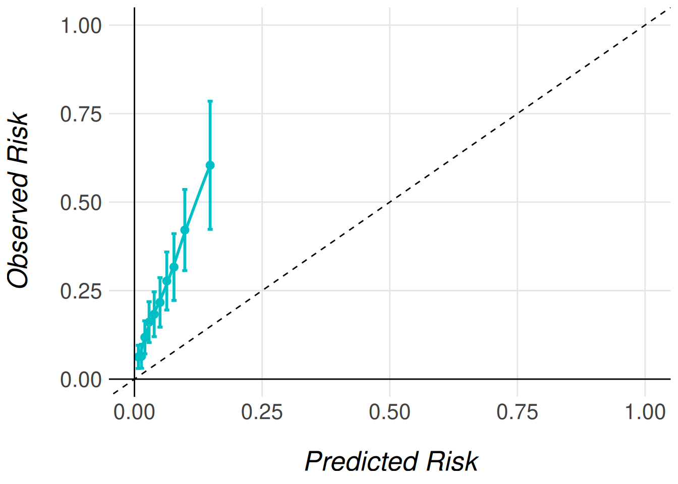
Calculating Calibration Plot
The calibration plots help users to visualize how accurate are the model predictions to the observed risks. To calculate the calibration plots it is mandatory to have calculated before the model predictions or their recalibration if needed. The package provides the user with some functions that allow them to generate the calibration plots.
The calibration plot calculation is divided into two steps, first step calculates the data where observed and predicted risks are represented. The observed risk can be calculated in different ways, in the package we have defined two function that allow the users to calculate them. The MiceExtVal::get_calibration_plot_data_surv() function calculates the observed risk by a Kaplan-Meier estimator and the MiceExtVal::get_calibration_plot_data_prop() function that calculates the observed risk as the proportion of events. From this data the calibration plot can be generated using the MiceExtVal::get_calibration_plot() function. The following code snippet shows how to calculate the calibration plots for the Framingham models.
men_model |>
  MiceExtVal::get_calibration_plot_data_surv(
    data = men_fram_long,
    n_groups = 10,
    type = "prediction"
  ) |>
  MiceExtVal::get_calibration_plot()

women_model |>
  MiceExtVal::get_calibration_plot_data_surv(
    data = women_fram_long,
    n_groups = 10,
    type = "prediction"
  ) |>
  MiceExtVal::get_calibration_plot()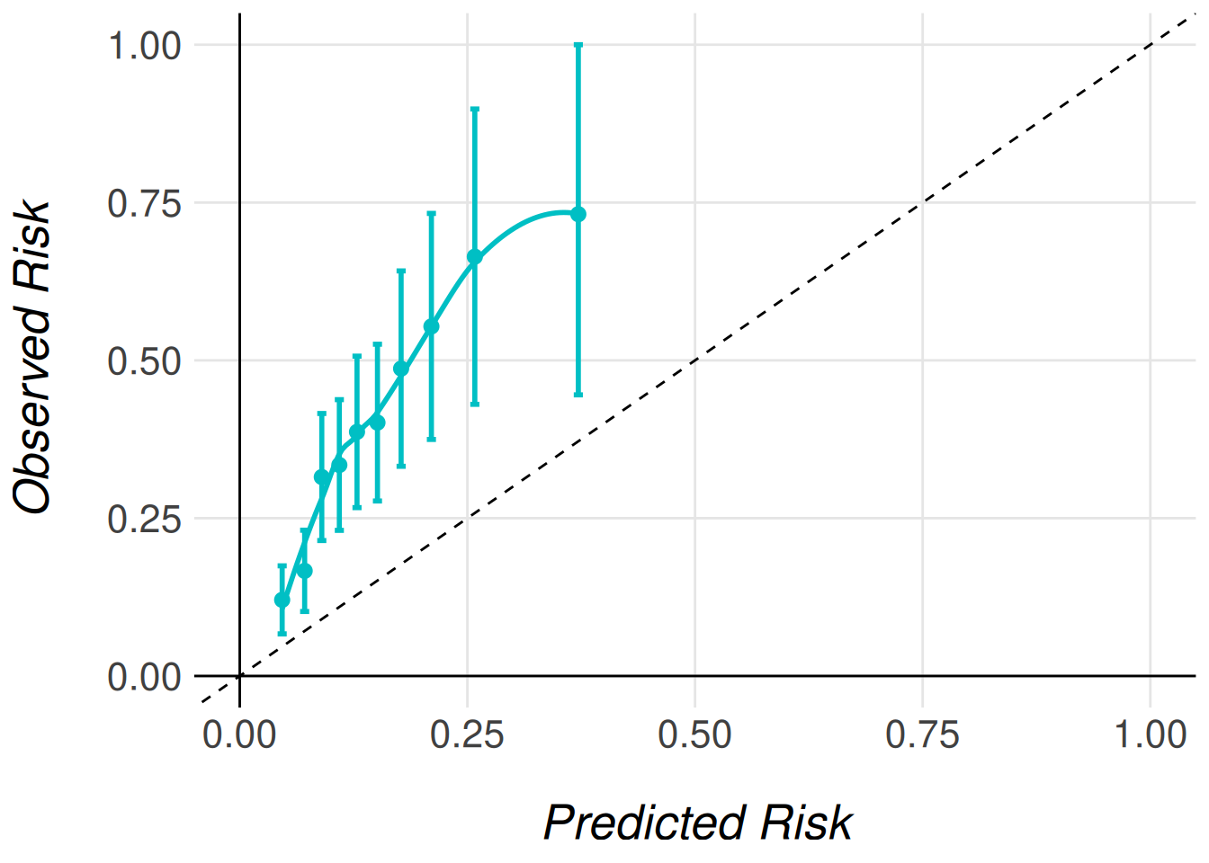
The calibration plots are a ggplot object and they can be modified as any other plot of the ggplot2 package. Feel free to modify them to match your requirements.
Calculation Brier Score
The Brier score is an statistic that measure the accuracy between the predicted riska and the observed outcome. In survival analysis we do no have an observed risk for each of the patients. Nevertheless we can assume that the outcome is dichotomous and calculate the Brier score with this type of outcome. The statistic is calculated as:
\[ BS = \frac{1}{N}\sum^N_{t = 1}(f_t - o_t)^2 \]
where \(N\) is the size of the population, \(f_t\) is the model prediction for the patient \(t\) y \(o_t\) is the observed risk for the patient \(t\) in this case \(0\) if they suffer no event and \(1\) otherwise.
In the MiceExtVal package we have developed the function MiceExtVal::calculate_brier_score that help users to calculate the model brier score.
men_model <- men_model |>
  MiceExtVal::calculate_brier_score(
    data = men_fram_long, type = "prediction", n_boot = 100
  )

women_model <- women_model |>
  MiceExtVal::calculate_brier_score(
    data = women_fram_long, type = "prediction", n_boot = 100
  )
dplyr::bind_rows(
  men_model[["results_agg"]] |> dplyr::filter(name == "brier_score"),
  women_model[["results_agg"]] |> dplyr::filter(name == "brier_score")
) |>
  tibble::add_column(Model = c("Men", "Women"), .before = "estimate") |>
kableExtra::kbl(digits = 3)| name | Model | estimate | lower | upper | p_val |
|---|---|---|---|---|---|
| brier_score | Men | 0.255 | 0.239 | 0.270 | - |
| brier_score | Women | 0.183 | 0.171 | 0.195 | - |
In Table 6 there are represented the brier score results for both models. It is important to remark that they are not comparable between them as they are calculated over different subcohorts of the framingham complete cohort.
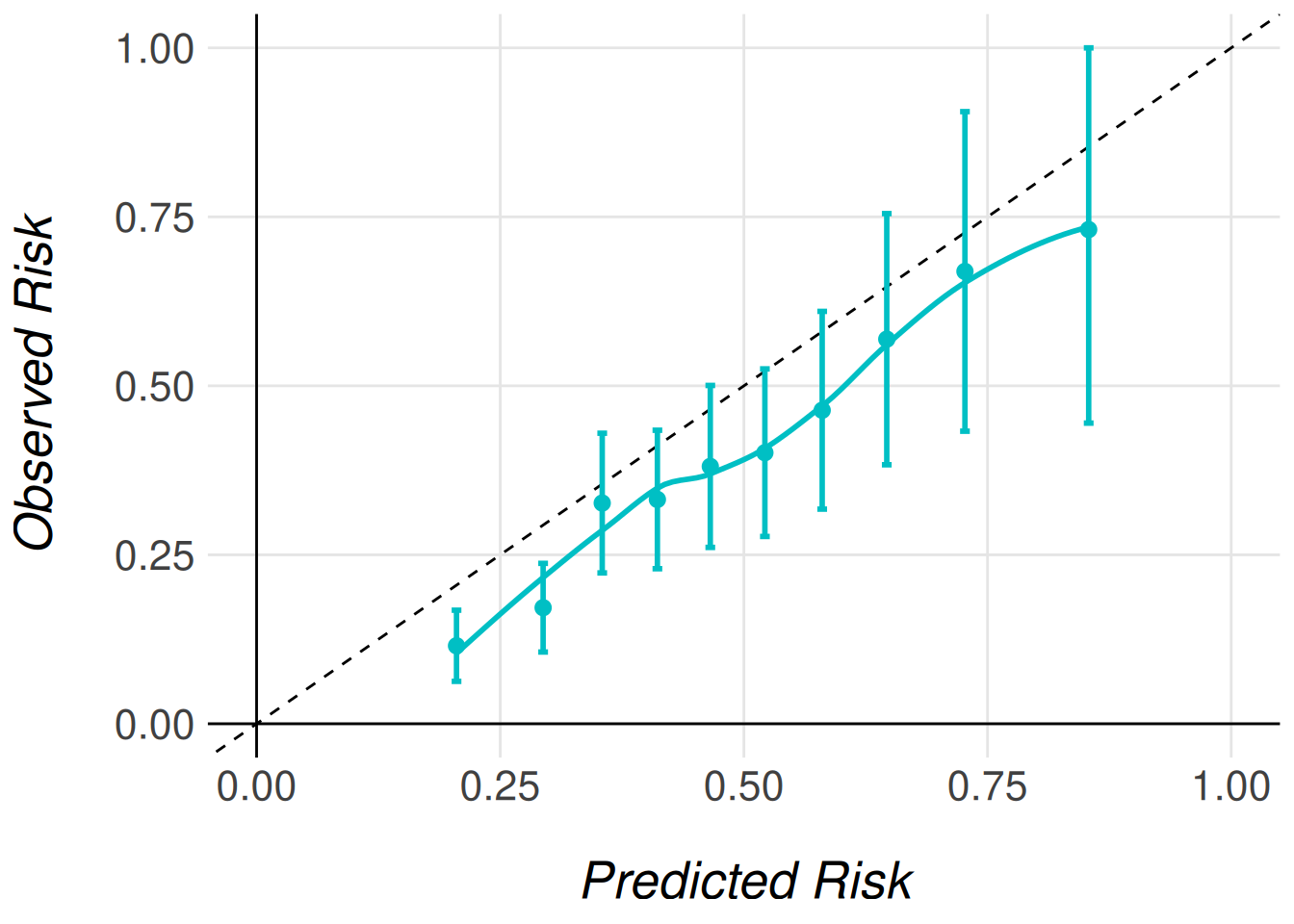
Recalibration
When we are validating a model in an external cohort is common that the model predictions do not match the observed risks in the new cohort. To minimize this problem we have developed two functions that allow the users to recalibrate the model predictions (please refer to MiceExtVal::calculate_predictions_recalibrated_type_1() and MiceExtVal::calculate_predictions_recalibrated_type_2() documentation for more detailed information on how the recalibration works).
men_model <- men_model |>
  MiceExtVal::calculate_predictions_recalibrated_type_1(data = men_fram_long) |>
  MiceExtVal::calculate_predictions_recalibrated_type_2(data = men_fram_long)

men_model |>
  MiceExtVal::get_calibration_plot_data_surv(
    data = men_fram_long,
    n_groups = 10,
    type = "prediction_type_1"
  ) |>
  MiceExtVal::get_calibration_plot()

men_model |>
  MiceExtVal::get_calibration_plot_data_surv(
    data = men_fram_long,
    n_groups = 10,
    type = "prediction_type_2"
  ) |>
  MiceExtVal::get_calibration_plot()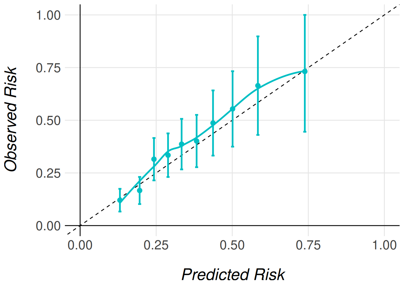
women_model <- women_model |>
  MiceExtVal::calculate_predictions_recalibrated_type_1(data = women_fram_long) |>
  MiceExtVal::calculate_predictions_recalibrated_type_2(
    data = women_fram_long
  )

women_model |>
  MiceExtVal::get_calibration_plot_data_surv(
    data = women_fram_long,
    n_groups = 10,
    type = "prediction_type_1"
  ) |>
  MiceExtVal::get_calibration_plot()

women_model |>
  MiceExtVal::get_calibration_plot_data_surv(
    data = women_fram_long,
    n_groups = 10,
    type = "prediction_type_2"
  ) |>
  MiceExtVal::get_calibration_plot()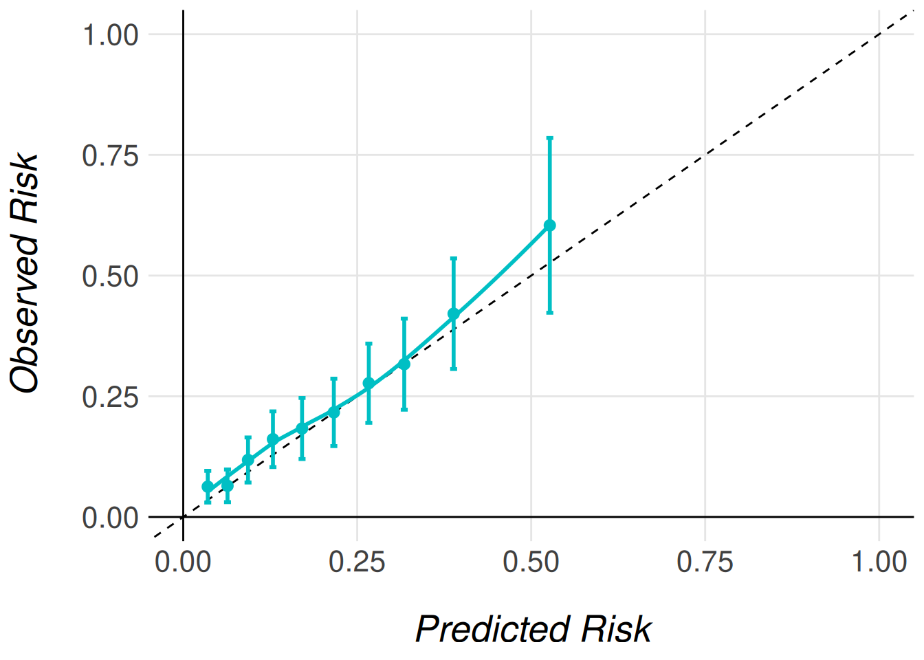
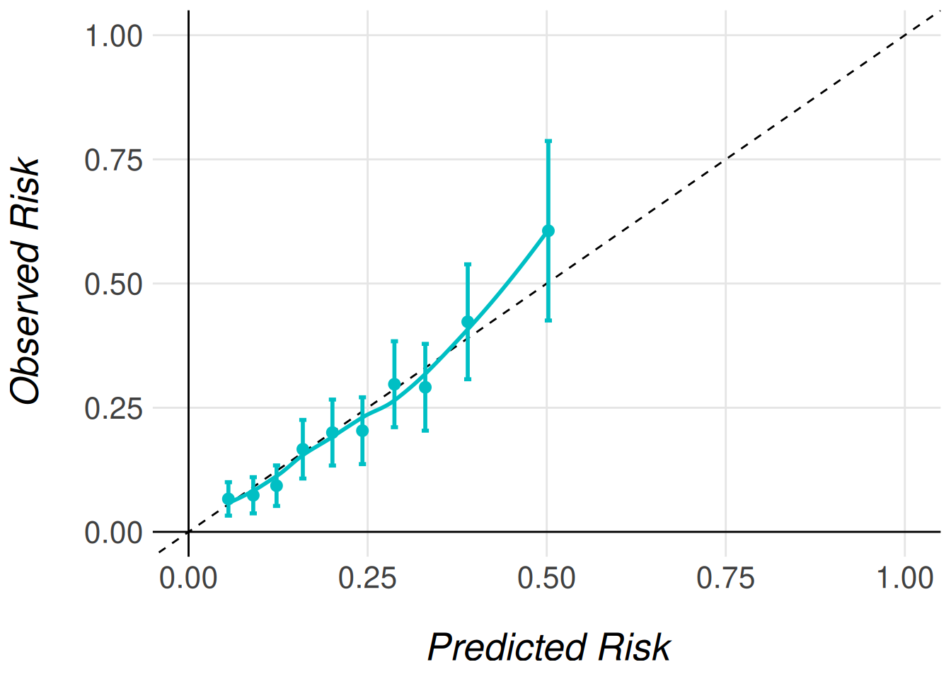
Type 1 and type 2 recalibration are not consecutive, they are just two different approaches for the same problem. As show in Figure 2, Figure 3 they obtain similar results. With the recalibration it also changes the Brier score results as shown in Table 7.
men_model <- men_model |>
  MiceExtVal::calculate_brier_score(
    data = men_fram_long, type = "prediction_type_1", n_boot = 100
  ) |>
  MiceExtVal::calculate_brier_score(
    data = men_fram_long, type = "prediction_type_2", n_boot = 100
  )

women_model <- women_model |>
  MiceExtVal::calculate_brier_score(
    data = women_fram_long, type = "prediction_type_1", n_boot = 100
  ) |>
  MiceExtVal::calculate_brier_score(
    data = women_fram_long, type = "prediction_type_2", n_boot = 100
  )

dplyr::bind_rows(
  men_model[["results_agg"]] |> dplyr::filter(name == "brier_score_type_1"),
  women_model[["results_agg"]] |> dplyr::filter(name == "brier_score_type_1")
  ) |>
  tibble::add_column(Model = c("Men", "Women"), .before = "estimate") |>
  kableExtra::kbl(digits = 3)
dplyr::bind_rows(
  men_model[["results_agg"]] |> dplyr::filter(name == "brier_score_type_2"),
  women_model[["results_agg"]] |> dplyr::filter(name == "brier_score_type_2")
  ) |>
  tibble::add_column(Model = c("Men", "Women"), .before = "estimate") |>
kableExtra::kbl(digits = 3)| name | Model | estimate | lower | upper | p_val |
|---|---|---|---|---|---|
| brier_score_type_1 | Men | 0.254 | 0.240 | 0.268 | - |
| brier_score_type_1 | Women | 0.184 | 0.171 | 0.198 | - |
| name | Model | estimate | lower | upper | p_val |
|---|---|---|---|---|---|
| brier_score_type_2 | Men | 0.254 | 0.238 | 0.269 | - |
| brier_score_type_2 | Women | 0.184 | 0.173 | 0.199 | - |
Comparing results
External validations are normally performed to compare different model performances among a certain cohort. The MiceExtVal package also provides users with functions that allow to compare results of different models.
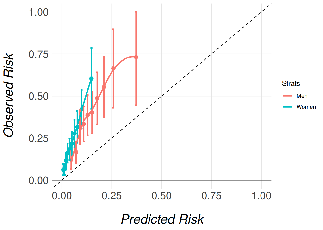
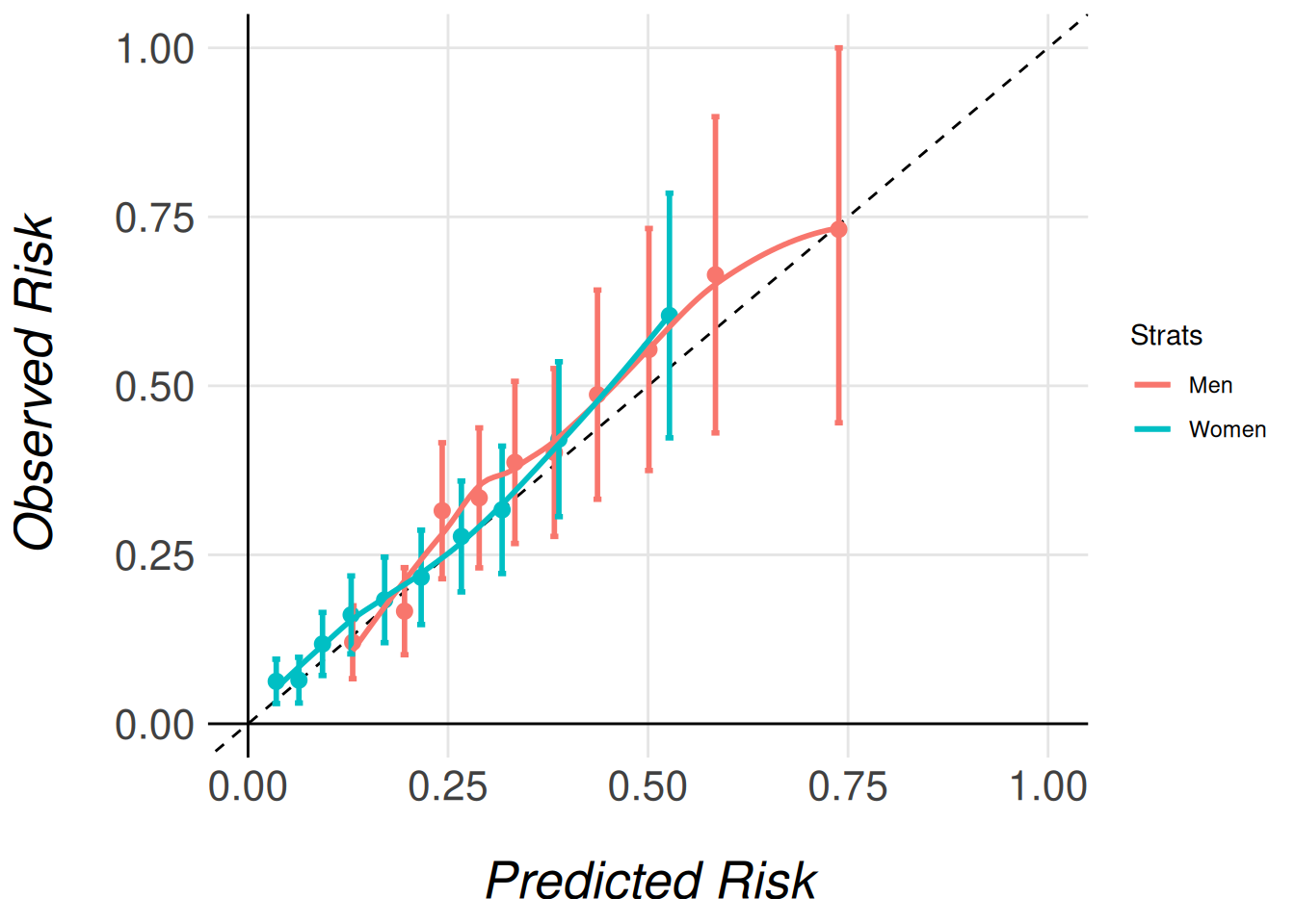
Calibration Comparison: Stratified Calibration Plots
In order to compare two model calibration plots we have developed the functions MiceExtval::get_stratified_calibration_plot_surv() and MiceExtval::get_stratified_calibration_plot_prop() that allow the user to plot stratified calibration plots. Accordingly with the individual calibration plots we use the function MiceExtval::get_stratified_calibration_plot_surv() to generate the stratified calibration plot.
In our case it could be interesting to plot men and women calibrations in the same plot, as shown in Figure 4. The function takes three arguments and a list of models as arguments.
- The external validation data (e.g.,
fram_long) - The number of groups
- The type of prediction (either recalibrated or original predictions)
- A list of models to compare (in this case,
men_modelandwomen_model).
This will allow the function to overlay calibration plots for both models on the same figure, facilitating direct comparison.
MiceExtVal::get_stratified_calibration_plot_surv(
  data = fram_long,
  n_groups = 10,
  type = "prediction",
  Men = men_model,
  Women = women_model
)

MiceExtVal::get_stratified_calibration_plot_surv(
  data = fram_long,
  n_groups = 10,
  type = "prediction_type_1",
  Men = men_model,
  Women = women_model
)

MiceExtVal::get_stratified_calibration_plot_surv(
  data = fram_long,
  n_groups = 10,
  type = "prediction_type_2",
  Men = men_model,
  Women = women_model
)
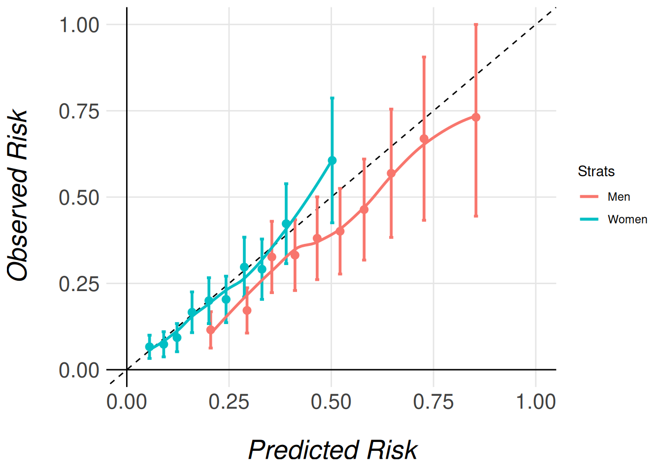
Note that we pass the entire imputed dataset (fram_long) as an argument, even though each model only stores the results for its respective subcohort (men or women). This is necessary because the function needs access to the full dataset in order to correctly extract and process the relevant subcohort for each model. The function then uses the subcohort specified for each model (e.g., men_model for men) to calculate the appropriate calibration data and generate the corresponding calibration plots.
By passing the complete dataset, the function ensures that the stratified calibration plots are generated correctly, comparing the models’ calibration in the context of the full cohort’s distribution of characteristics.
Discrimination Comparison: Forestplot
The MiceExtVal package also includes functionality for generating a forest plot to compare the discrimination abilities of different models. In this example, we will visualize the Harrell C-Index, but the package also allows for the comparison of the AUC (Area Under the Curve) in dichotomous outcomes.
The forest plot generation process is split into two steps:
- Data preparation: The first step generates the data that will be used in the forest plot.
- Forest plot creation: The second step generates the actual plot from the prepared data.
To compare different models, we can stratify the results by binding data from different subgroups (e.g., men and women patients). Models that share the same name across subgroups will be merged in the final forest plot, making it easy to compare the performance of the same model in different groups.
In the following example, we generate two separate strata for the same model, TIMI-II, one for men and one for women, and then we pass these strata to the forest plot function.
dplyr::bind_rows(
  MiceExtVal::get_forestplot_data(
    strat = "Men", type = "harrell_c_index", Framingham = men_model
    ),
  MiceExtVal::get_forestplot_data(
    strat = "Women", type = "harrell_c_index", Framingham = women_model
    )
) |>
MiceExtVal::get_forestplot(center = 0.7, digits = 2) |
|||
| Model | Men (95% CI) | Women (95% CI) | |
|---|---|---|---|
| Framingham | 0.69 (0.66, 0.71) | 0.71 (0.69, 0.74) |  |
 |
|||
If we want to generate a forestplot with multiple models in one strat we can generate it as the following example. In this example men and women models are inserted in the Overall strat as individual models. We have deleted the legend as it is not informative.
MiceExtVal::get_forestplot_data(
  strat = "Overall",
  type = "harrell_c_index",
  `Framingham Women` = women_model,
  `Framingham Men` = men_model
) |>
MiceExtVal::get_forestplot(center = 0.7, digits = 2) |
||
| Model | Overall (95% CI) | |
|---|---|---|
| Framingham Women | 0.71 (0.69, 0.74) |  |
| Framingham Men | 0.69 (0.66, 0.71) |  |
|
||
Brier Score Comparison: Forestplot
The forestplot functions also allow us to generate the data from the Brier score results. The next code snippet generates a forestplot that compares the different Brier score in each model.
data <- dplyr::bind_rows(
  MiceExtVal::get_forestplot_data(
    strat = "Original", type = "brier_score",
    Men = men_model, Women = women_model
  ),
  MiceExtVal::get_forestplot_data(
    strat = "Type 1 recalibration", type = "brier_score_type_1",
    Men = men_model, Women = women_model
  ),
  MiceExtVal::get_forestplot_data(
    strat = "Type 2 recalibration", type = "brier_score_type_2",
    Men = men_model, Women = women_model
  ),
)

data |>
  MiceExtVal::get_forestplot(
    center = mean(data[["estimate"]]),
    digits = 2,
    axis.text.x = ggplot2::element_text(size = 25)
) |
||||
| Model | Original (95% CI) | Type 1 recalibration (95% CI) | Type 2 recalibration (95% CI) | |
|---|---|---|---|---|
| Men | 0.26 (0.24, 0.27) | 0.25 (0.24, 0.27) | 0.25 (0.24, 0.27) |  |
| Women | 0.18 (0.17, 0.20) | 0.18 (0.17, 0.20) | 0.18 (0.17, 0.20) |  |
 |
||||